Introduction to Assembly

• Since the processor can only process binary data “i.e. 1’s and 0’s”, it would be challenging for humans to interact with processors without referring to manuals to know which hex code runs which instruction.
• This is where Assembly language comes in, as a low-level language that can write direct instructions the processors can understand.
• By using Assembly, developers can write human-readable machine instructions, which are then assembled into their machine code equivalent, so that the processor can directly run them.
• For example, the Assembly code 'add rax, 1' is much more intuitive and easier to remember than its equivalent machine shellcode '4883C001', and easier to remember than the equivalent binary machine code '01001000 10000011 11000000 00000001'.
• As we can see, without Assembly language, it is very challenging to write machine instructions or directly interact with the processor.

Compilation Stages

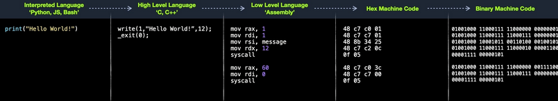
• Let’s take a basic ‘Hello World!’ program that prints these words on the screen and show how it changes from high-level to machine code.
• In an interpreted language, like Python, it would be the following basic line:

  print("Hello World!")
  

• If we run this Python line, it would be essentially executing the following C code:

  #include <unistd.h>
  int main(){
    write(1,"Hello World!",12); // 1-> stdout
    _exit(0);
  }
  

• The above C code uses the Linux write syscall, built-in for processes to write to the screen. The same syscall called in Assembly looks like the following:

  mov rax,1
  mov rdi,1
  mov rsi,message
  mov rdx,12
  syscall
  mov rax,60
  mov rdi,0
  syscall
  

• As we can see, when the write syscall is called in C or Assembly, both are using 1, the text, and 12 as the arguments.
• The previous Assembly code can be assembled into the following hex machine code (i.e., shellcode):

  48 c7 c0 01
  48 c7 c7 01
  48 8b 34 25
  48 c7 c2 0c
  0f 05
  48 c7 c0 3c
  48 c7 c7 00
  0f 05
  

• Finally, for the processor to execute the instructions linked to this machine, it would have to be translated into binary, which would look like the following:

  01001000 11000111 11000000 00000001
  01001000 11000111 11000111 00000001
  01001000 10001011 00110100 00100101
  01001000 11000111 11000010 00001100 
  00001111 00000101
  

• A CPU uses different electrical charges for a 1 and a 0, and hence can calculate these instructions from the binary data once it receives them.

Value for Pentesters

• Understanding assembly language instructions is critical for binary exploitation, which is an essential part of penetration testing.
• To disassemble, debug, and follow binary instructions in memory and find potential vulnerabilities, we must have a basic understanding of Assembly language and how it flows through the CPU components.
• NB: Learning Intel x86 Assembly Language is crucial for writing exploits for binaries on modern machines.
• In addition to Intel x86, ARM is becoming more common, as most modern smartphones and some modern laptops like the M1 MacBook Pro feature ARM processors.

Computer Architecture

• This architecture executes machine code to perform specific algorithms. It mainly consists of the following elements:
  • Central Processing Unit (CPU)
  • Memory Unit
  • Input/Output Devices
• Furthermore, the CPU itself consists of three main components:
  • Control Unit (CU)
  • Arithmetic Logic Unit (ALU)
  • Registers
    
• Though very old, this architecture is still the basis of most modern computers, servers, and even smartphones.
• Assembly languages mainly work with the CPU and memory.
• Furthermore, basic and advanced binary exploitation requires a proper understanding of computer architecture.
  • With basic stack overflows, we only need to be aware of the general design.
  • Once we start using ROP and Heap exploits, our understanding should be profound.

Memory

• A computer’s memory (Primary Memory) is where the temporary data and instructions of currently running programs are located.
• It is the primary location the CPU uses to retrieve and process data.
• There are two main types of memory:
  • Cache
  • Random Access Memory (RAM)
• Cache memory is usually located within the CPU itself and hence is extremely fast compared to RAM, as it runs at the same clock speed as the CPU.
  • However, it is very limited in size and very sophisticated, and expensive to manufacture due to it being so close to the CPU core.
  • There are usually three levels of cache memory, depending on their closeness to the CPU core:

  Level	Description
  Level 1 Cache	Usually in kilobytes, the fastest memory available, located in each CPU core. (Only registers are faster.)
  Level 2 Cache	Usually in megabytes, extremely fast (but slower than L1), shared between all CPU cores.
  Level 3 Cache	Usually in megabytes (larger than L2), faster than RAM but slower than L1/L2. (Not all CPUs use L3.)

• RAM
• RAM is much larger than cache memory, coming in sizes ranging from gigabytes up to terabytes.
• RAM is also located far away from the CPU cores and is much slower than cache memory.
• Accessing data from RAM addresses takes many more instructions.
• In the past, with 32-bit addresses, memory addresses were limited from 0x00000000 to 0xffffffff.
• This meant that the maximum possible RAM size was 232 bytes, which is only 4 gigabytes, at which point we run out of unique addresses.
• With 64-bit addresses, the range is now up to 0xffffffffffffffff, with a theoretical maximum RAM size of 264 bytes, which is around 18.5 exabytes (18.5 million terabytes), so we shouldn’t be running out of memory addresses anytime soon.
• When a program is run (done), all of its data and instructions are moved from the storage unit to the RAM to be accessed when needed by the CPU.
• The RAM is split into 4 segments:
  

Segment	Description
Stack	Has a Last-in First-out (LIFO) design and is fixed in size. Data in it can only be accessed in a specific order by push-ing and pop-ing data.
Heap	Has a hierarchical design and is therefore much larger and more versatile in storing data (Meaning the data could be stored any where), as data can be stored and retrieved in any order. However, this makes the heap slower than the Stack.
Data	Has to parts: Data, which is used to hold variables, .bss, which is used to hold unassigned variables (i.e., buffer memory for later allocation).
Text	Main assembly instructions are loaded into this segment to be fetched and executed by the CPU.

CPU Architecture

• The Central Processing Unit (CPU) is the main processing unit within a computer.
• The CPU contains both the ,
  • Control Unit (CU) Which is in charge of moving and controlling data, and the
  • Arithmetic/Logic Unit (ALU), which is in charge of performing various arithmetics and logical calculations as requested by a program through the assembly instructions.
• The manner in which and how efficiently a CPU processes its instructions depends on its Instruction Set Architecture (ISA).
  • RISC architecture is based on processing more simple instructions, which takes more cycles, but each cycle is shorter and takes less power.
  • CISC architecture is based on fewer, more complex instructions, which can finish the requested instructions in fewer cycles, but each instruction takes more time and power to be processed.

Clock speed & Clock cycle

• Each CPU has a clock speed that indicates its overall speed.
• The frequency in which the cycles occur is counted, is cycles per second (Hertz).
• If a CPU has a speed of 3.0 GHz, it can run 3 billion cycles every second (per core).
  
  
• Instruction Cycle:
  • An instruction cycle is the cycle the CPU takes to process a single machine instruction.
    
    
    
• An instruction cycle consists of four stages: Fetch, Decode, Execute, and Store:

Instruction	Description
1. Fetch	Takes the next instruction's address from the Instruction Address Register (IAR), which tells it where the next instruction is located.
2. Decode	Takes the instruction from the IAR, and decodes it from binary to see what is required to be executed.
3. Execute	Fetch instruction operands from register/memory, and process the instruction in the ALU or CU.
4. Store	Store the new value in the destination operand.

All of the stages in the instruction cycle are carried out by the Control Unit, except when arithmetic instructions need to be executed “add, sub, ..etc”, which are executed by the ALU.

• Each Instruction Cycle takes multiple clock cycles to finish, depending on the CPU architecture and the complexity of the instruction.
• Once a single instruction cycle ends, the CU increments to the next instruction and runs the same cycle on it, and so on.
  
  
  
• For example, if we were to execute the assembly instruction add rax, 1, it would run through an instruction cycle:
  1. Fetch the instruction from the rip register, 48 83 C0 01 (in binary).
  2. Decode ‘48 83 C0 01’ to know it needs to perform an add of 1 to the value at rax.
  3. Execute: Get the current value at rax (by CU), add 1 to it (by the ALU).
  4. Store the new value back to rax.
• In the past, processors used to process instructions sequentially, so they had to wait for one instruction to finish to start the next.
• On the other hand, modern processors can process multiple instructions in parallel by having multiple instruction/clock cycles running at the same time.
• This is made possible by having a multi-thread and multi-core design.
  
  
  

Processor Specific

It is important to understand that each processor has its own set of instructions and corresponding machine code.

• Even though we can tell that both instructions are similar and do the same thing, their syntax is different, and the locations of the source and destination operands are swapped as well. Still, both codes assemble the same machine code and perform the same instruction.
• So, each processor type has its Instruction Set Architectures, and each architecture can be further represented in several syntax formats
• If we want to know whether our Linux system supports x86_64 architecture, we can use the lscpu command:
  • Manual:
    
    
  • Usage:
    
    

• We can also use the uname -m command to get the CPU architecture.
  
  

Instruction Set Architectures

• An Instruction Set Architecture (ISA) specifies the syntax and semantics of the assembly language on each architecture.
• ISA mainly consists of the following components:
  • Instructions
  • Registers
  • Memory Addresses
  • Data types
    

Component	Description	Example
Instruction	The instruction to be processed in the opcode operand_list format. There are usually 1,2, or 3 comma-separated operands.	add rax, 1,mov rsp, rax, push rax
Registers	Used to store operands, addresses, or instructions temporarily.	rax, rsp, rip
Memory Addresses	The address in which data or instructions are stored. May point to memory or registers.	0xffffffffaa8a25ff, 0x44d0, $rax
Data Types	The type of stored data.	byte, double word, word

• There are two main Instruction Set Architectures that are widely used:
  • Complex Instruction Set Computer (CISC) - Used in Intel and AMD processors in most computers and servers.
  • Reduced Instruction Set Computer (RISC) - Used in ARM and Apple processors, in most smartphones, and some modern laptops.

    CISC

• The CISC architecture was one of the earliest ISA’s ever developed.
• CISC architecture favors more complex instructions to be run at a time to reduce the overall number of instructions.
  • For example, suppose we were to add two registers with the ‘add rax, rbx’ instruction.
  • In that case, a CISC processor can do this in a single ‘Fetch-Decode-Execute-Store’ instruction cycle, without having to split it into multiple instructions to fetch rax, then fetch rbx, then add them, and then store them in `rax, each of which would take its own ‘Fetch-Decode-Execute-Store’ instruction cycle.
• Furthermore, even though it takes a single instruction cycle to execute a single instruction, as the instructions are more complex, each instruction cycle takes more clock cycles. This fact leads to more power consumption and heat to execute each instruction.

RISC

• The RISC architecture favors splitting instructions into minor instructions, and so the CPU is designed only to handle simple instructions.
• For example, the same previous add r1, r2, r3 instruction on a RISC processor would fetch r2, then fetch r3, add them, and finally store them in r1.
  • Every instruction of these takes an entire ‘Fetch-Decode-Execute-Store’ instruction cycle, which leads, as can be expected, to a larger number of total instructions per program, and hence a longer assembly code.
• The below diagram shows how CISC instructions take a variable amount of clock cycles, while RISC instructions take a fixed amount:
  
  
  
• CISC vs. RISC

Area	CISC	RISC
Complexity	Favors complex instructions.	Favors simple instructions
Length of instructions	Longer instructions - Variable length 'multiples of 8-bits'	Shorter instructions - Fixed length '32-bit/64-bit'
Total instructions per program	Fewer total instructions - Shorter code	More total instructions - Longer code
Optimization	Relies on hardware optimization (in CPU)	Relies on software optimization (in Assembly)
Instruction Execution Time	Variable - Multiple clock cycles	Fixed - One clock cycle
Instructions supported by CPU	Many instructions (~1500)	Fewer instructions (~200)
Power Consumption	High	Very Low
Examples	Intel and AMD	ARM, Apple

Registers, Addresses, and Data Types

• Now that we understand general computer and processor architecture, we need to understand a few assembly elements before we start learning Assembly: Registers, Memory Addresses, Address Endianness, and Data Types.
• Each of these elements is important, and properly understanding them will help us avoid issues and hours of troubleshooting while writing and debugging assembly code.

Registers

• As previously mentioned, each CPU core has a set of registers.
• The registers are the fastest components in any computer, as they are built within the CPU core.
• However, registers are very limited in size and can only hold a few bytes of data at a time.
• There are two main types of registers we will be focusing on: Data Registers and Pointer Registers.

Data Registers	Pointer Registers
rax	rbp
rbx	rsp
rcx	rip
rdx
r8
r9
r10

• Data Registers: are usually used for storing instructions/syscall arguments. The primary data registers are: rax, rbx, rcx, and rdx. The rdi and rsi registers also exist and are usually used for the *instruction destination and source operands*. Then, we have secondary data registers that can be used when all previous registers are in use, which are r8, r9, and r10.
• Pointer Registers: are used to store specific important address pointers. The main pointer registers are the Base Stack Pointer rbp, which points to the beginning of the Stack, the Current Stack Pointer rsp, which points to the current location within the Stack (top of the Stack), and the Instruction Pointer rip, which holds the address of the next instruction.

Sub-Registers

• Each 64-bit register can be further divided into smaller sub-registers containing the lower bits, at one byte 8-bits, 2 bytes 16-bits, and 4 bytes 32-bits.
• Each sub-register can be used and accessed on its own, so we don’t have to consume the full 64-bits if we have a smaller amount of data.
  
  
• Sub-registers can be accessed as:
  

Size in bits	Size in bytes	Name	Example
16-bit	2-bytes	the base name	ax
8-bit	1-byte	the base name + and/or ends with l	al
32-bits	4-bytes	the base name + and/or starts with e prefix	eax
64-bits	8-bytes	the base name + and/or starts with r prefix	rax

• For example, for the bx data register, the 16-bit is bx, so the 8-bit is bl, the 32-bit is eax, and the 64-bit would be rbx.
• This also applies to the base and stack pointers:
  • It’s sub-register bpl is an 8-bit
  • The register bp is a 16-bit (base name)
  • The register ebp is a 32-bit
  • The register rbp is a 64-bit
  • The above is the same for stack pointer.
• The RFLAGS register in the x86_64 architecture is a 64-bit status register that contains condition flags reflecting the outcome of various CPU operations.
• Flags include:
  • Carry Flag (CF): Indicates carry or borrow in arithmetic operations.
  • Zero Flag (ZF): Set if the result of an operation is zero.
  • Sign Flag (SF): Reflects the sign of the result (negative or positive).
  • Overflow Flag (OF): Set if signed overflow occurs.
  • Interrupt Enable Flag (IF): Controls whether interrupts are enabled.
  • Direction Flag (DF): Controls string operation direction.
  • Parity Flag (PF): Indicates even parity of the least significant byte.

Memory Addresses

• x86_64-bit processors have 64-bit wide addresses that range from 0x0 to 0xffffffffffffffff
• There are several types of address fetching (i.e., addressing modes) in the x86 architecture:
  

Addressing Mode	Description	Example
Immediate	The value is given within the instruction	ADD 7
Register	The register name that holds a value is given in the instruction.	ADD eax
Direct	The direct full address is given in the instruction.	ADD 0xffffffffaa8a25ff
Indirect	A reference pointer is given in the instruction.	CALL 0x44d000 or CALL [rax]
Stack	The address is on top of the stack	ADD rsp

Address Endianness

• An address endianness is the order of its bytes in which they are stored or retrieved from memory.
• There are two types of endianness: Little-Endian and Big-Endian.
• With Little-Endian processors, the little-end byte of the address is filled/retrieved first right-to-left, while with Big-Endian processors, the big-end byte is filled/retrieved first left-to-right.
  
  
• When retrieving the value, the processor has to use the same endianness used when storing them, or it will get the wrong value.
• NB:
  • Intel/AMD which are 86_64-bit architecture use Little Endian:
  • The important thing we need to take from this is knowing that our bytes are stored into memory from right-to-left.

Data Types

• The following are the most common data types we will be using with instructions:

Component	Length	Example
byte	8-bits	0xab
word	16-bits (2-bytes)	0xabcd
double word (dword)	32-bits (4-bytes)	0xabcdef12
quad word (qword)	64-bits (8-bytes)	0xabcdef1234567890

“Whenever we use a variable with a certain data type or use a data type with an instruction, both operands should be of the same size.”

• For example, we cannot use a variable of data type (byte) with rax as it is of data type 8-bytes; Hence in this case for a byte we have to use al which has the same size of 1 byte.

Sub-Register	Data Type
al	byte
bx	word
ebx	dword
rbx	qword

Assemble File Structure

• Assembly code template:

        global _start
  
        section .data
  message: db     "Hello World"
  
        section .text
  _start:
        mov     rax,1
        mov     rdi,1
        mov     rsi,message
        mov     rdx,18
        syscall 
  
        mov     rax,60
        mov     rdi,0
        syscall
  

• First, let’s examine the way the code is distributed:
  
• Looking at the vertical parts of the code, each line can have three elements:

 1. Labels      2. Instructions      3. Operands 

• Next, if we look at the code line-by-line, we see that it has three main parts:

section .dataThis is the data section, which should contain all of the variables.

Section	Description
_global start	This is a directive that directs the code to start executing at the _start label defined below.
section .text	This is the text section containing all of the code to be executed.

• directives:
  • An Assembly code is line-based, which means that the file is processed line-by-line, executing the instruction of each line.
  • We see at the first line a directive global _start, which instructs the machine to start processing the instructions after the _start label.
• Variables:
  • Next, we have the .data section.
  • The data section holds our variables to make it easier for us to define variables and reuse them without writing them multiple times.
  • Once we run our program, all of our variables will be loaded into memory in the data segment.
  • We can define variables using db for a list of bytes, dw for a list of words, dd for a list of digits, and so on.
  • Furthermore, we can use the equ instruction with the $ token to evaluate an expression, like the length of a defined variable’s string.
    • However, the labels defined with the equ instruction are constants, and they cannot be changed later.
  • For example, the following code defines a variable and then defines a constant for its length:

      section .data
      message db "Hello world!", 0x0a
      length  equ $-message
    

    • Note: the $ token indicates the current distance from the beginning of the current section.
    • As the message variable is at the beginning of the data section, the current location, i.e,. value of $, equals the length of the string.
• Code:
  • This section holds all of the assembly instructions and loads them to the text memory segment.
  • Once all instructions are loaded into the text segment, the processor starts executing them one after another.
  • The default convention is to have the _start label at the beginning of the .text section, which -as per the global _start directive- starts the main code that will be executed as the program runs.
  • The text segment within the memory is read-only, so we cannot write any variables within it.
  • The data section, on the other hand, is read/write, which is why we write our variables to it.
  • However, the data segment within the memory is not executable, so any code we write to it cannot be executed.
  • This separation is part of memory protections to mitigate things like buffer overflows and other types of binary exploitation.

    Tip: We can add comments to our assembly code with a semi-colon ;. We can use comments to explain the purpose of each part of the code, and what each line is doing. Doing so will save us a lot of time in the future if we ever revisit the code and need to understand it.

Assemble & Disassemble

Assemble

• we can assemble our code with nasm, we can link it using ld to utilize various OS features and libraries.
• Hence the following assembly code:
  
  
• And to assemble the code (Note: The -f elf64 flag is used to note that we want to assemble a 64-bit assembly code. If we wanted to assemble a 32-bit code, we would use -f elf.):

  nasm -f elf64 basic.s
  

• This should output a basic.o object file, which is then assembled into machine code, along with the details of all variables and sections. This file is not executable just yet.
• Linking
  • The final step is to link our file using ld.
  • The basic.o object file, though assembled, still cannot be executed.
  • This is because many references and labels used by nasm need to be resolved into actual addresses, along with linking the file with various OS libraries that may be needed.
  • FUN FACT: This is why a Linux binary is called ELF, which stands for an Executable and Linkable Format.
  • To link a file using ld, we can use the following command:

      ld -o basic.o basic
    

Disassembling

• To disassemble a file, we will use the objdump tool, which dumps machine code from a file and interprets the assembly instruction of each hex code.
• We can disassemble a binary using the -d flag.
• Note: we will also use the flag -M intel, so that objdump would write the instructions in the Intel syntax, which we are using, as we discussed before (note the difference below).
  
  
• from above we see that; nasm efficiently changed our 64-bit registers to the 32-bit sub-registers where possible, to use less memory when possible, like changing mov rax, 1 to mov eax,0x1.
• The -d flag will only disassemble the .text section of our code.
• To dump any strings, we can use the -s flag, and add -j .data to only examine the .data section (This means that we also do not need to add -M intel).
  
  
• Flag:
  

GNU Debugger (GDB)

• Programs written in high-level languages can set breakpoints on specific lines and run the program through a debugger to monitor how they act.
• With Assembly, we deal with machine code represented as assembly instructions, so our breakpoints are set in the memory location in which our machine code is loaded.
• To debug our binaries, we will be using a well-known debugger for Linux programs called GNU Debugger (GDB).
• There are other similar debuggers for Linux, like Radare and Hopper, and for Windows, like Immunity Debugger and WinGDB.
  
  
• As we can see, the output we got closely resembles our assembly code and the disassembly output we got from objdump in the previous section.
• Having the memory address is critical for examining the variables/operands and setting breakpoints for a certain instruction.
• You may notice through debugging that some memory addresses are in the form of 0x00000000004xxxxx, rather than their raw address in memory 0xffffffffaa8a25ff
  • This is due to $rip-relative addressing in Position-Independent Executables (PIE), in which the memory addresses are used relative to their distance from the instruction pointer $rip within the program’s own Virtual RAM, rather than using raw memory addresses.
  • This feature may be disabled to reduce the risk of binary exploitation.

Debugging with GDB

• Now that we have the general information about our program, we will start running it and debugging it.
• Debugging consists mainly of four steps:

Step	Description
Break	Setting breakpoints at various points of interest.
Examine	Running the program and examining the state of the program at these points
Step	Moving through the program to examine how it acts with each instruction and with user input
Modify	Modify values in specific registers or addresses at specific breakpoints, to study how it would affect the execution

Break

• The first step of debugging is setting breakpoints to stop the execution at a specific location or when a particular condition is met.
• This helps us in examining the state of the program and the value of registers at that point.
• Breakpoints also allow us to stop the program’s execution at that point so that we can step into each instruction and examine how it changes the program and values.
• We can set a breakpoint at a specific address or for a particular function.
• To set a breakpoint, we can use the break or b command along with the address or function name we want to break at.
• If we want to set a breakpoint at a certain address, like _start+10, we can either b *_start+10 or b *0x40100a:
• The * tells GDB to break at the instruction stored in 0x40100a.
• NB: Once the program is running, if we set another breakpoint, like b *0x401005, in order to continue to that breakpoint, we should use the continue or c command. If we use run or r again, it will run the program from the start. This can be useful to skip loops, as we will see later in the module.
• If we want to see what breakpoints we have at any point of the execution, we can use the info breakpoint command.
• We can also disable, enable, or delete any breakpoint.

Examine

• The next step of debugging is examining the values in registers and addresses.
• To manually examine any of the addresses or registers or examine any other, we can use the x command in the format of x/FMT ADDRESS, as help x would tell us.
• The ADDRESS is the address or register we want to examine, while FMT is the examine format.
• The examine format FMT can have three parts:

Argument	Description	Example
Count	The number of times we want to repeat the examine	3,4,8
Format	The format we want the result to be represented in	x(hex), s(string), i(instruction)
Size	The size of memory we want to examine	b(byte), h(halfword), w(word), g(giant, 8 bytes)

• Instruction:
  • if we wanted to examine the next four instructions in line, we will have to examine the $rip register (which holds the address of the next instruction), and use 4 for the count, i for the format, and g for the size (for 8-bytes or 64-bits).
    
  • We see that we get the following four instructions as expected.
  • This can help us as we go through a program in examining certain areas and what instructions they may contain.
• Strings:
  • We can also examine a variable stored at a specific memory address.
  • We know that our message variable is stored at the .data section on address 0x402000 from our previous disassembly.
  • We also see the upcoming command movabs rsi, 0x402000, so we may want to examine what is being moved from 0x402000.
  • In this case, we will not put anything for the Count, as we only want one address (1 is the default), and will use s as the format to get it in a string format rather than in hex:
    
  • As we can see, we can see the string at this address represented as text rather than hex characters.
• Addresses
  • We often need to examine addresses and registers containing hex data, such as memory addresses, instructions, or binary data.
  • Let us examine the same previous instruction, but in hex format, to see how it looks:
    
  • We see instead of mov eax,0x1, we get 0x000001b8, which is the hex representation of the mov eax,0x1 machine code in little-endian formatting.
    • This is read as: b8 01 00 00.
• Step
  • The third step of debugging is stepping through the program one instruction or line of code at a time.
  • As we can see, we are currently at the very first instruction in our basic program:
    
  • Note: the instruction shown with the -> symbol is where we are at, and it has not yet been processed.
  • To move through the program, there are three different commands we can use: stepi, step and s.
  • The stepi or si command will step through the assembly instructions one by one, which is the smallest level of steps possible while debugging.
  • Let us use the si command to see how we get to the next instruction:
    
  • As we can see, we took exactly one step and stopped again at the mov edi, 0x1 instruction.
• Step Count
  • Similarly to examine, we can repeat the si command by adding a number after it.
  • For example, if we wanted to move 3 steps to reach the syscall instruction, we can do so as follows:
    
  • As we can see, we stopped at the syscall instruction as expected.
  • You can hit the return/enter empty in order to repeat the last command. Try hitting it at this stage, and you should make another 3 steps, and break at the other syscall instruction.
    
    
• Step
  • The step or s command, on the other hand, will continue until the following line of code is reached or until it exits from the current function.
  • If we run an assembly code, it will break when we exit the current function _start
  • If there’s a call to another function within this function, it’ll break at the beginning of that function.
  • Otherwise, it’ll break after we exit this function after the program’s end.
  • Let us try using s, and see what happens:
    
  • We see that the execution continued until we reached the exit from the _start function, so we reached the end of the program and exited normally without any errors.
  • There’s also the next or n command, which will also continue until the next line, but will skip any functions called in the same line of code, instead of breaking at them like step. There’s also the nexti or ni, which is similar to si, but skips functions calls.
    
• Modify
  • The final step of debugging is modifying values in registers and addresses at a certain point of execution.
  • This helps us in seeing how this would affect the execution of the program.
  • Addresses:
    • To modify values in GDB, we can use the set command.
    • However, we will utilize the patch command in GEF to make this step much easier.
    • Let’s enter help patch in GDB to get its help menu:
      
    • As we can see, we have to provide the type/size of the new value, the location to be stored, and the value we want to use.
    • So, let’s try changing the string stored in the .data section (at address 0x402000 as we saw earlier) to the string Yo Katt we winning!\n.
      
    • Notice how we used \x0a for adding a new line after our string.
• Registers
  • We also note that we did not replace the entire string.
  • This is because we only modified the characters up to the length of our string and left the remainder of the old string.
  • Finally, the write system call specified a length of 0x12 of bytes to be printed.
  • To fix this, let’s modify the value stored in $rdx to the length of our string, which is 0x9.
    

Data Movement

• The main Data Movement instructions are:

Instruction	Description	Example
mov	Move data or load immediate data	mov rax,1=> rax=1
lea	Load an address pointing to the value	lea rax,[rsp+5]=> rax=rsp+5
xchg	Swap data between two registers or addresses	xchg rax,rbx=> rax=rbx, rbx=rax

• Moving Data
• Address Pointers
  • In many cases, we would see that the register or address we are using does not immediately contain the final value but contains another address that points to the final value.
  • We can use square brackets to compute an address offset relative to a register or another address. For example, we can do mov rax, [rsp+10] to move the value stored 10 address away from rsp.
• Loading Value Pointers
  • Finally, we need to understand how to load a pointer address to a value, using the lea (or Load Effective Address) instruction, which loads a pointer to the specified value, as in lea rax, [rsp].
  • This is the opposite of what we just learned above (i.e., load pointer to a value vs. move value from pointer).
  • This is usually done when the data is large and would not fit in one register, so the data is placed on the stack or in the heap, and a pointer to its location is stored in the register.
  • Note that if we use mov rax, [rsp+10], it will actually move the value at [rsp+10] to rax, as discussed earlier. We cannot move a pointer with an offset using mov.

Arithmetic Instructions

• With Arithmetic Instructions, we can perform various mathematical computations on data stored in registers and memory addresses.
• These instructions are usually processed by the ALU in the CPU, among other instructions.
• We will split arithmetic instructions into two types: instructions that take only one operand (Unary), instructions that take two operands (Binary).
• Unary Instructions:
  • The following are the main Unary Arithmetic Instructions (we will assume that rax starts as 1 for each instruction):

Instruction	Description	Example
inc	Increment by 1	inc rax -> rax++ or rax += 1 -> rax = 2
dec	Decrement by 1	dec rax -> rax-- or rax -= 1 -> rax = 0

• Binary Instructions:
  • Next, we have Binary Arithmetic Instructions, and the main ones are: We’ll assume that both rax and rbx start as 1 for each instruction.
  • The following are the main Unary Arithmetic Instructions (we will assume that rax starts as 1 for each instruction):

Instruction	Description	Example
add	Add both operands	add rax, rbx -> rax = 1 + 1 -> 2
sub	Subtract Source from Destination (i.e rax = rax - rbx)	sub rax, rbx -> rax = 1 - 1 -> 0
imul	Multiply both operands	imul rax, rbx -> rax = 1 * 1 -> 1

• Bitwise Instructions:
  • Now, let’s move to Bitwise Instructions, which are instructions that work on the bit level (we’ll assume that rax = 1 and rbx = 2 for each instruction):

Instruction	Description	Example
not	Bitwise NOT (invert all bits, 0->1 and 1->0)	not rax -> NOT 00000001 -> 11111110
and	Bitwise AND (if both bits are 1 -> 1, if bits are different -> 0)	and rax, rbx -> 00000001 AND 00000010 -> 00000000
or	Bitwise OR (if either bit is 1 -> 1, if both are 0 -> 0)	or rax, rbx -> 00000001 OR 00000010 -> 00000011
xor	Bitwise XOR (if bits are the same -> 0, if bits are different -> 1)	xor rax, rbx -> 00000001 XOR 00000010 -> 00000011

Loops

• Loop Structure:
  • A loop in assembly is a set of instructions that repeat for rcx times. Let’s take the following example:

      exampleLoop:
      instruction 1
      instruction 2
      instruction 3
      instruction 4
      instruction 5
      loop exampleLoop
    

  • Once the assembly code reaches exampleLoop, it will start executing the instructions under it.
  • We should set the number of iterations we want the loop to go through in the rcx register.
  • Every time the loop reaches the loop instruction, it will decrease rcx by 1 (i.e., dec rcx) and jump back to the specified label, exampleLoop in this case.
  • So, before we enter any loop, we should mov the number of loop iterations we want to the rcx register.

Instruction	Description	Example
mov rcx, x	Sets loop (rcx) counter to x	mov rcx, 3
loop	Jumps back to the start of loop until counter reaches 0	loop exampleLoop

Unconditional Branching

• The second type of Control Instructions is Branching Instructions, which are general instructions that allow us to jump to any point in the program if a specific condition is met.
• Let’s first discuss the most basic branching instruction:
  • jmp, which will always jump to a location unconditionally.
  • The jmp instruction jumps the program to the label or specified location in its operand so that the program’s execution is continued there.
  • Once a program’s execution is directed to another location, it will continue processing instructions from that point.
  • The basic jmp instruction is unconditional, which means that it will always jump to the specified location, regardless of the conditions.
  • unconditional jumps completely redirect execution - they don’t execute any instructions between the jump and the target label!
  • This contrasts with Conditional Branching instructions that only jump if a specific condition is met:

Instruction	Description	Example
jmp	Jumps to specified label, address, or location	jmp loop

Conditional Branching

• Unlike Unconditional Branching Instructions, Conditional Branching instructions are only processed when a specific condition is met, based on the Destination and Source operands.
• A conditional jump instruction has multiple varieties as Jcc, where cc represents the Condition Code.
• The following are some of the main condition codes:

Instruction	Condition	Example
jz	D = 0	Destination equal to Zero
jnz	D != 0	Destination Not equal to Zero
js	D < 0	Destination is Negative
jns	D >= 0	Destination is Not Negative (i.e. 0 or positive)
jg	D > S	Destination Greater than Source
jge	D >= S	Destination Greater than or Equal Source
jl	D < S	Destination Less than Source
jle	D <= S	Destination Less than or Equal Source

RFLAGS Register

• The RFLAGS register consists of 64-bits like any other register. However, this register does not hold values but holds flag bits instead.
• Each bit ‘or set of bits’ turns to 1 or 0 depending on the value of the last instruction.

• Just like other registers, the 64-bit RFLAGS register has a 32-bit sub-register called EFLAGS, and a 16-bit sub-register called FLAGS, which holds the most significant flags we may encounter.

• The flags we would mostly be interested in are:
  • The Carry Flag CF: Indicates whether we have a float.
  • The Parity Flag PF: Indicates whether a number is odd or even.
  • The Zero Flag ZF: Indicates whether a number is zero.
  • The Sign Flag SF: Indicates whether a register is negative.
• JNZ loopFib:
  • Though it is more efficient to use loop, to demonstrate the use of jnz, let’s go back to our code and try to use the jnz instruction instead of loop:

      gobal _start
      section .text
      _start:
      mov rax,0
      mov rbx,0
      inc rbx
      mov rcx,10
      loopFib:
      add rax,rbx
      xchg rax,rbx
      dec rcx
      jnz loopFib
    

  • Every time the loop reaches its end, the rcx counter would decrement by 1, and the program would jump back to loopFib if ZF is not set.
  • Once rcx reaches 0, the Zero Flag ZF would be turned on to 1, and so jnz would no longer jump (since it’s NZ), and we would exit the loop.
    

CMP

• The Compare instruction cmp simply compares the two operands, *by subtracting the second operand from first operand (i.e. D1 - S2), and then sets the necessary flags in the RFLAGS register.
• For example, if we use cmp rbx, 10, then the compare instruction would do ‘rbx - 10’, and set the flags based on the result.

Instruction	Description	Example
cmp	Sets RFLAGS by subtracting second operand from first operand (i.e. first - second)	cmp rax, rbx -> rax - rbx

• The main advantage of ‘cmp’ is that it does not affect the operands.
• Note: In a cmp instruction, the first operand (i.e. the Destination) must be a register, while the other can be a register, a variable, or an immediate value.

Using the Stack

• Before we discuss Functions, we need to understand how to use the memory Stack.
• The Stack:
  • The stack is a segment of memory allocated for the program to store data in, and it is usually used to store data and then retrieve them back temporarily.
  • The top of the stack is referred to by the Top Stack Pointer rsp, while the bottom is referred to by the Base Stack Pointer rbp.
  • NB: We can push data into the stack, and it will be at the top of the stack (i.e. rsp), and then we can pop data out of the stack into a register or a memory address, and it will be removed from the top of the stack.

Instruction	Description	Example
push	Copies the specified register/address to the top of the stack	push rax
pop	Moves the item at the top of the stack to the specified register/address	pop rax

• The stack has a Last-in First-out (LIFO) design, which means we can only pop out the last element pushed into the stack.

Usage With Functions/Syscalls

• We will primarily be pushing data from registers into the stack before we call a function or call a syscall, and then restore them after the function and the syscall.
• For example, if we wanted to call a syscall to print Hello World to the screen and retain the current value stored in rax, we would push rax into the stack.
• Then we can execute the syscall and afterward pop the value back to rax.
• So, this way, we would be able to both execute the syscall and retain the value of rax.
• Using the stack is very simple. The only thing we should keep in mind is the order we push our registers and the state of the stack to safely restore our data and not restore a different value by pop when a different value is at the top of the stack.

Syscalls

• A syscall is like a globally available function written in C, provided by the Operating System Kernel.
• A syscall takes the required arguments in the registers and executes the function with the provided arguments.
• For example, if we wanted to write something to the screen, we can use the write syscall, provide the string to be printed and other required arguments, and then call the syscall to issue the print.
• There are many available syscalls provided by the Linux Kernel, and we can find a list of them and the syscall number of each one by reading the unistd_64.h system file:
  
• The above file sets the syscall number for each syscall to refer to that syscall using this number.
• Note: With 32-bit x86 processors, the syscall numbers are in the unistd_32.h file.

Syscall Function Arguments

• To use the write syscall, we must first know what arguments it accepts.
• To find the arguments accepted by a syscall, we can use the man -s 2 command with the syscall name from the above list:
  
• As we can see from the above output, the write function has the following syntax: Code (highlighted part):
  
• We see that the syscall function expects 3 arguments:
  • File Descriptor fd to be printed to (usually 1 for stdout)
  • The address pointer to the string to be printed.
  • The length we want to print.
• Once we provide these arguments, we can use the syscall instruction to execute the function and print to screen.

Syscall Calling Convention

• Now that we understand how to locate various syscall and their arguments let’s start learning how to call them. To call a syscall, we have to:
  • Save registers to stack
  • Set its syscall number in rax
  • Set its arguments in the registers
  • Use the syscall assembly instruction to call it
• We usually should save any registers we use to the stack before any function call or syscall.
• Syscall Number:
  • Let’s start by moving the syscall number to the rax register.
  • As we saw earlier, the write syscall has a number 1, so we can start with the following command:

      mov rax, 1